Difference between revisions of "Move Tatrabot 2D mapping - Johanna, Romana, Nicole, Oswaldo, Dušan, Viktor"
(→Movement and Navigation) |
m (→Sensors) |
||
| Line 140: | Line 140: | ||
== Sensors == | == Sensors == | ||
| − | |||
| − | |||
| − | |||
| − | |||
| − | |||
| − | |||
| − | |||
| − | |||
| − | |||
| − | |||
| − | |||
| − | |||
| − | |||
| − | |||
| − | |||
| − | |||
| − | |||
| − | |||
| − | |||
=== Ultrasonic Measurement System === | === Ultrasonic Measurement System === | ||
| Line 197: | Line 178: | ||
* Weight 8.5g | * Weight 8.5g | ||
| + | |||
| + | === Rotation Sensors === | ||
| + | |||
| + | Robot is capable of performing 3 distinct moves. After each move the position in map is being updated. | ||
| + | |||
| + | '''Forward''' | ||
| + | |||
| + | First we force robot to move past line it stands in front of. Then robot starts moving forward tracking the line. If it changed heading (because of any reasons), it corrects it’s heading. If robot turns left, left motor moves while right stops. If it turns right, left motor stops while right corrects heading. If sensor on far right sees the line, it means we traveled far enough (to next perpendicular line), so we set both motors to reverse to get before line again and cycle can repeat. | ||
| + | |||
| + | '''Right''' | ||
| + | |||
| + | At first, left motor makes 90 degree turn (to right). Then both motors reverse and after that robot uses forward method to find line and stop in front of it. | ||
| + | |||
| + | '''Left''' | ||
| + | |||
| + | Robot moves forward past the line and starts backing with left motor only. Then it moves in a reverse for some more fixed distance and looks for a line with forward method again. | ||
| + | |||
| + | All of these moves move robot to the same position, slightly to the right of the line just in front of next line perpendicular to direction of robot. Therefore these moves can be chained indefinitely. | ||
== STM32 platform == | == STM32 platform == | ||
Revision as of 00:29, 29 June 2018
The project's aim was to let the Tatrabot successfully reach a given target position in a grid environment using A* search algorithm. This is realized by creating an internal two-dimensional-map representing the robot's current position in the environment and its knowledge about probable locations of obstacles, gained from taking ultrasonic measurements during movement. To account for inaccurate movements Tatrabot uses its LED-sensors to perceive and follow the grid's lines.
Contents
Grid to Map Representation
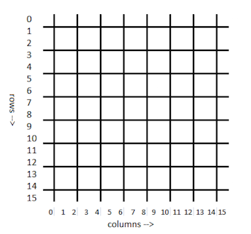
An 8 by 8 grid of 20 by 20cm squares with 2.5cm black borders was printed out as the layout of the map over which the robot is to navigate. This corresponded to a 16 by 16 (row, column) coordinate system as shown in the figure below.
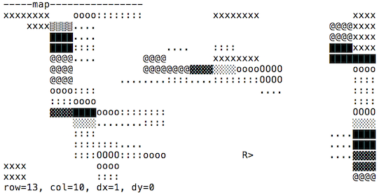
To represent the grid layout with obstacle arrangement and the movement of the robot within it, 3 virtual maps were constructed. Data was collected by the robot searching through the map using A* searching algorithm. Constant signals from the ultrasonic sensors were received. The position of the robot within the map is represented by an "R" followed by an arrow " < , > ,^ or v " corresponding to the orientation of the robot. The following are the 3 constructed maps. The figures illustrate the state of the maps at the same moment in time.
See Obstacle Map
-----see obstacle----------------
 0   0   0   1   1   1   0   0   0   0   0   0   0   0   0   0
 0   0   0  20  15   1   0   0   0   0   0   2   2   5  14   0
 0   0   1  54  57  11  13   0   0   1   1   1   0   3  12   0
 0   0   1  52  46   0   0   0   0  25   0   0   1   4  12   0
 0   0   0  28  14   0  24   2   0   8   0  14   1   2  12   0
 0   0  11   9   0   0   1   3   0   0   0   9   1   1   0   0
 0   0  11   9   0   0   0  21  83  83  47   3   0   0   0   0
 0   0  18  16   0   0   0  35  81  81  34  14   1   0   2  11
 0   0  18  16   0   0   0   1   4   5   5   1   1   0   2  11
 0   0  18  18   7   7   0   0   1   2   1   1   1   0  18  13
 0   0   7  54   3   3  11  10  10   0   0   1   1  18  24   4
 0   0   7  75  39  39  24   1   1   0   0   0   0  18  22   3
 0   0   0  49  57  24  Rv  13  13   0   0   0   0  18   6  54
 0   0   0   7  46   1   1   1   1   1   0   2   2   2   2  55
 0   0   0   8 106   1   0   0   0   0   0   3   3   3   3 115
 0   0   0   2  61   2   1   0   0   0   0   1   1   1   1  60
The see obstacle map is a map of how many times an obstacle has been sensed in that particular position. Depending on the detected distance of the object, the radius of the ultrasonic beam at that distance is calculated. The algorithm then takes into consideration the width of the cells and the orientation of the robot to determine which cells fall within that radius. The value representing the probability of the obstacle is then incremented within those cells.
The position and orientation of the robot within the grid is not an absolute one but is tracked and changed depending on the initial position and orientation and the respective changes in position and orientation. The direction of signal detection is also changed accordingly.
See Nothing Map
-----see nothing-----------------
 0   0   0  11  11  11   0   0   0  18  18  39  65  65  47   0
33   3   3  15  34  34  22   0   0  33  33  54  80  77  21   0
33  33   5  19  62 108  69  84  51  69  55  55  82  79  23   4
65  33   5  30  73 119  69  84  51  76  62  62  87  83   4   4
35  35   3  27  69  83   9  15  15  34  34  25  54  53   4  13
41  32   0  11  61  61  34  40  15  24  43  34  84  83  13  13
 9   9   0  11 104 104  45  54  30  21  40  28  53  53  13  13
31  31  22  18  71  71  36  65 109  84  41  31  95  95  70  38
22  22  22  40 103 103  83  83 155 171 242  63 105 105 112  80
41  41  41  55  85  85  72  72 163 167  87  82 124 124 106  72
19  19  19  51 119 119 122  60 233 252  19  40  97  79  55  50
19  19  19  31  57  57  75  36 126 252  19  19  77  59  37  13
 0   0   0   7  77  87  Rv  42  80  79  22  43  74  93  87  12
 0   0   0  33  40  86 101  61  79 101  22  41  72  72  72  19
 0   0   0  32  39  91 109  61  20  42  22  38  75 255 255  16
 0   0   0  30  30 111 108  61  20  42  22  37  74  74  74  15
The see nothing map increments the probability of " no obstacle" in the cells in front of the detected object. It also increments the "no obstacle" probability of cells within a 154cm distance where no obstacle is detected. The radius of the ultrasonic beam is also taken into consideration as in the "see obstacle" map.
Full Map
It is estimated, due to the angle of the obstacles with respect to the robot, the material and reflectance of the obstacle, and the general sensitivity of the sensors, that an obstacle is only detected about 1/5 of the time. To compensate for this inconsistency, therefore, the value of the "see obstacle" map only needs to be 1/5 that of the "see nothing" map in order to be considered as present.
The probability of an obstacle being present is further represented in increments using UTF-8 characters to create a better visualization of the map. It is calculated by dividing the number of times an obstacle was perceived at the given location by the sum of measurements taken from this location.
Implementation of A* Algorithm
Function initialize_plan_data_structures
Initialize the data that will be used to make a plan to go from a starting position to a final position.
Data structures:
- Array of visited blocks by the robot which initially have value 0 for every block except for the block where the robot currently is (value 1).
- A start point in the queue initialized with 0.
- An end point in the queue initialized with 1.
Function insert_into_queue
Inserts values for rows and columns in a queue according to the plan until the starting value of the queue is the same as the ending value.
Data structures:
- Array of rows in queue and columns in queue.
- Starting and ending values of the queue.
Function create_plan
Creates a valid plan, executes initialize_plan_data_structures and while the ending value in the queue is higher than the starting value it assigns the rows and columns in the queue to the current values of the rows and columns. Then it tries a direction forwards or backwards in columns as well as in rows. The algorithm will try to find a suitable route to the goal without leaving the map, avoiding obstacles, and not visiting already visited spaces on the grid. If the space on the grid is suitable for the robot to move there, the function will assign a visited value on that space and sum that movement into the count of the steps from start, and the visited value will be inserted in the queue. When the candidate row and column reaches the destination row and column the queue starting point will have reached the ending point of the queue, meaning that all the points in the queue correspond to the route from start to goal. Finally, it plans the direction in which the robot will move and the corresponding rows and columns through steps. It adds the steps required to go to the goal and it calculates the plan length.
Data structures:
- Array of suitable directions.
- Array of candidate rows and columns.
- Array of visited rows and columns.
- Steps from start based on the candidate rows and columns.
- Plan length based on steps from start.
Coordinate Systems
The robot is using 3 coordinates systems:
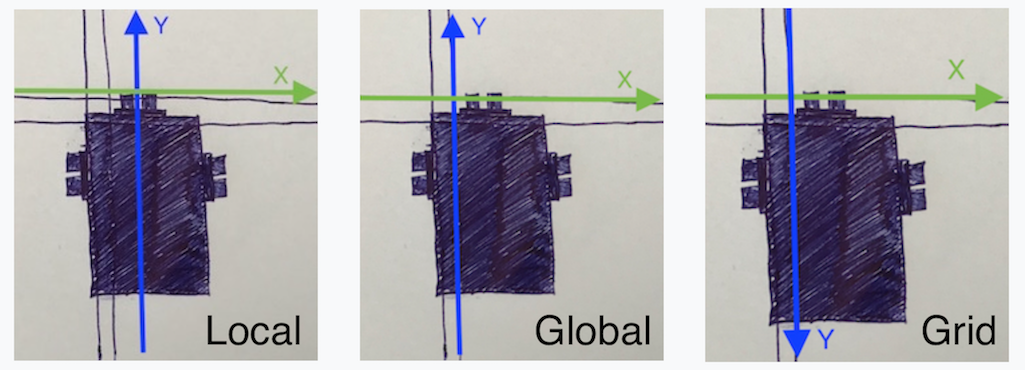
- Local
- Global
- Grid
Every ultrasonic sensor has its own local coordinate system. The point [0,0] is oriented in front of each sensor, the X-coordinate is growing from left to right and the Y-coordinate is rising from down to top in the direction of the sensor.
The global coordinate system is used for real calculation. It’s a normal mathematics coordinate system. Each sensor has defined his own shift from global point [0,0].
The grid coordinate system is the last one, which is used for grid representation of the map. The X-coordinate is the same, but the Y-coordinate is switched. This is because a representation of map is stored in a 2-dimensional array. Every point in the real grid is represented as 4 points in our array.
The final calculation is provided on global coordinate system using shifts and final result of seen and unseen is done with vector transformation to grid coordinate system.
Ultrasonic Sensor Model
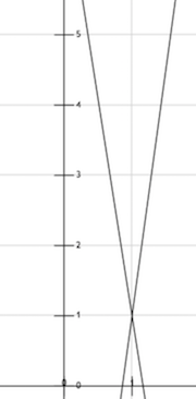
The cone is defined by the following 2 functions (see also figure on the right):
These functions are used to determine if any point is in the cone. The condition is met when the result of first function is in interval (-∞;0> and of second in interval <0; ∞).
The process to update seen and unseen is described like this:
- Get measurement of sensor as distance
- Processing every row from robot position until distance as unseen
- Updating columns in row to the left until at least 1 condition is matched:
- is in cone left distant edge
- is in cone right distant edge
- the cone is between left and right distant edge
- Same updating columns in row to the right as to the left
- Mark all columns as seen at distance with same process
This process is done for every used sensor with its own measured distance.
Sensors
Ultrasonic Measurement System
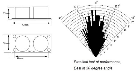
Our robot is equiped with 3 HCSRO4P ultrasonic sensors.
Their general directions are:
- Front
- Left
- Right
Sensors are being run in endless loop measuring distances in all 3 directions working through 18 states. There are 6 states for each sensor direction.
- sets value 1 on pin GPIOB13
- clears GPIO13 pid
- waits for value on GPIO12, starting bit
- waits until sensor stops transmitting on GPIO12, which signals that measuring stopped. If transmission doesnt stop until 870ms, waiting stops and default value is used.
- is used as a state signaling that this sensor is already measured and other sensors can be used.
- means that measuring failed, response wasn’t recieved
States 1-6 work with sensor 1, while states 7-12 are used for sensor 2 and 13-18 for sensor 3.
HCSR04P module
This module is the second generation of HC-SR04 Ultrasonic Sensor. Unlike the first generation HC-SR04 that can only operate between 4.8V 5V DC, this new version has wider input voltage range, allow it to work with controller operates on 3.3V. It measures distance using sonar, an ultrasonic (well above human hearing) pulse (40KHz) is transmitted from the unit and distance-to-target is determined by measuring the time required for the echo return.
Features
- HC-SR04P Upgrade version with build-in crystal, more reliable, lower working current.
- Power Supply: 3.3 5 VDC
- Quiescent Current : <2mA
- Working Current: 2.8mA @ 5V
- Effective Angle: <15 degrees
- Ranging Distance : 2 to 400 cm
- Connector: 4-pins header with 2.54mm pitch.
- Dimension: 45mm x 20mm x 15mm
- Weight 8.5g
Rotation Sensors
Robot is capable of performing 3 distinct moves. After each move the position in map is being updated.
Forward
First we force robot to move past line it stands in front of. Then robot starts moving forward tracking the line. If it changed heading (because of any reasons), it corrects it’s heading. If robot turns left, left motor moves while right stops. If it turns right, left motor stops while right corrects heading. If sensor on far right sees the line, it means we traveled far enough (to next perpendicular line), so we set both motors to reverse to get before line again and cycle can repeat.
Right
At first, left motor makes 90 degree turn (to right). Then both motors reverse and after that robot uses forward method to find line and stop in front of it.
Left
Robot moves forward past the line and starts backing with left motor only. Then it moves in a reverse for some more fixed distance and looks for a line with forward method again.
All of these moves move robot to the same position, slightly to the right of the line just in front of next line perpendicular to direction of robot. Therefore these moves can be chained indefinitely.
STM32 platform
STM32 is a family of 32-bit microcontroller integrated circuits by STMicroelectronics. The STM32 chips are grouped into related series that are based around the same 32-bit ARM processor core, such as the Cortex-M7F, Cortex-M4F, Cortex-M3, Cortex-M0+, or Cortex-M0. Internally, each microcontroller consists of the processor core, static RAM memory, flash memory, debugging interface, and various peripherals.
Visual Studio
The aim of the Visual Studio code is to create a visualisation of the physical Tatrabot action. It generates a map with probable obstacles and marks the most efficient route to the final destination depending on the starting point, final destination and obstacles by utilizing the A* search. It helps us proceed the task faster than in real world.
It utilizes the following functions:
- fill_the_map creates a map consisting of number of rows and columns simulating the real field
- char robot_orientation marks the robots orientation at a current position with an arrow symbols and marks obstacles with the ‘’@’’ symbol
- print_level_of_gray visualises the magnitude of a probability of an obstacle occurrence at each spot separately
- initialize_plan_data_structures organises the data (starting point, destination and visited spots) needed for the evaluation of the plan
- insert_into_queue calculates values for each spot and inserts them into a queue
- create_plan finds the most appropriate route and creates plans length
- navigate_to executes and prints the calculated route, if the create_plan function didn’t find the suitable route, it prints "No trajectory exists.’’
