Comparing Reinforcement Learning with Neuroevolution - Tomáš Bisták
Contents
Problem Statement and Goal
This project aims to compare two optimization methods for training an agent to solve a sequential, Markovian decision task from robotics. More precisely, we assume to have a robotic arm with the tip of its end effector moving across a table. This robot's task is to use its end effector to push a small chip on the table to a desired location. We consider this task to be modeled as a Reinforcement-Learning (RL) problem. Our goal is to train agents via Advantage Actor-Critic (A2C) and NeuroEvolution of Augmenting Topologies (NEAT) and assess their performance.
Methods
We suppose the reader to be familiar with the frameworks of RL and Evolutionary Algorithms (EAs). For more details on these topics, please refer to the treatises from Sutton and Barto [1] and Eiben and Smith [2], respectively. We now briefly describe the two learning techniques we have evaluated.
Advantage Actor-Critic
Consider a discrete-time Markov Decision Process (MDP) M with a state space S \in R^n, an action space A \in R^m, and a dynamics function p: S x A -> S x R, which gives the probability p(s', r | s, a) of the next state s' \in S and the immediate reward r \in R for any given previous state s \in S and action taken a \in A. To find an optimal policy \pi^*, we cannot simply maintain a tabular approximation of the state- or action-value function (V_\pi or Q_\pi) for the current policy \pi since M has a continuous state space. Neither may we solely rely on parametrized representations of the value functions (v_w or q_w) such as Artificial Neural Networks (ANNs) because the action space of M is continuous as well.
The family of Advantage Actor-Critic (A2C) RL methods [1] thus works both with a parametrized state-value-function approximation v_w (a critic) and a parametrized policy \pi_\theta (an actor). The actor always decides the action to be chosen, even during training, which requires its policy to be soft, i.e., to be able to select each action with a non-zero probability. The training of (one-step) A2C resides in finding optimal parameters \theta online by performing the following pair of updates after each experienced transition from a state s \in S to a state s' \in S through an action a \in A yielding a reward r \in R:
   \theta <- \theta + \alpha * (r + \gamma * v_w(s') - v_w(s)) * \nabla_\theta ln(\pi_\theta(s)),
        w <- w + \beta * (r + \gamma * v_w(s') - v_w(s)) * \nabla_w v_w(s),
where \alpha, \beta \in [0, 1] are learning rates and \gamma \in [0, 1] is the discount factor. Intuitively, this algorithm makes a small step in the direction of the observed advantage of taking the selected action – r + \gamma * v_w(s') - v_w(s) – after every decision.
Note that the above updates incorporate the inverse of pure Stochastic Gradient Descent (SGD), but A2C is also compatible with any of the more advanced versions of SGD (e.g., RMSProp or Adam).
NeuroEvolution of Augmenting Topologies
NeuroEvolution of Augmenting Topologies (NEAT) [3] is a general-purpose EA for simultaneously optimizing weights and topologies of ANNs. It evolves a population of ANNs divided into species based on their structural and weight differences. The initial population contains merely networks with no hidden neurons and a full wiring from inputs to outputs. Individuals with new nodes and connections are gradually introduced throughout evolution. More information about the process and the employed genetic operators can be found in [3].
Environment
We have prepared a Python simulation for our task's environment to train and test the agents. In this simplified model, the tabletop is assumed to be rectangular and to lie in the x-y plane, with the bottom left corner at (0, 0) and the top right at (1000, 700). The state is described by a vector of 6 values:
- the x position of the end effector's tip (the actuator, for short),
- the y position of the actuator,
- the x position of the chip relative to the actuator,
- the y position of the chip relative to the actuator,
- the x position of the goal position relative to the actuator,
- the y position of the goal position relative to the actuator.
The chip is modeled as a circle with a radius of chip_radius = 20, and the chip's position is given by the circle's center. Each action consists of a pair (dx, dy) \in [-1, 1]^2 determining the direction and the magnitude of the actuator's step in both axes. This vector is scaled by a factor of step_size = 10 before being applied. Hence, the agent only tells where the tip of the end effector should be moved, but not how. The step reward r \in R is calculated via the following procedure:
   procedure calculate_reward(p_a, p_c, p_g, p_a_last, p_c_last, p_g_last)
       r <- 1 / step_size * \Delta ||p_c - p_g||_2           # motivate moving the chip closer to the goal
       if ||p_c - p_g||_2 < chip_radius / 2 then
           r <- r + 0.1                                      # motivate keeping the chip close to the goal
       else
           r <- r + 1 / step_size * \Delta ||p_a - p_c||_2   # motivate moving the actuator closer to the chip

           dist_to_push <- (1 - <p_c - p_g, p_a - p_c>
                                / (||p_c - p_g||_2 * ||p_a - p_c||_2))
           if dist_to_push > 0.02 then
               r <- r + 2 * \Delta dist_to_push              # motivate pushing the chip directly to the goal
           end
       end
       if the actuator or a part of the chip is off the table then
           r <- r - 0.1                                      # deter from getting off the table
       end
       return r
   end procedure
where p_a, p_c, and p_g are the resulting positions of the actuator, the chip, and the goal, p_a_last, p_c_last, and p_g_last are the previous positions of the actuator, the chip, and the goal, \Delta e takes the difference between the expression e evaluated for the next and last positions, and <v_1, v_2> is the dot product of vectors v_1 and v_2.
To simplify the simulation of chip pushing, we have made several assumptions such as that this process is friction-free. We do not further cover the details of our implementation of pushing for brevity.
Experiments
We have conducted all experiments in our RL environment with an episode horizon of 1000 steps and \gamma = 0.99. We have implemented the A2C method ourselves and used the Python library NEAT-Python [4] to run slightly modified NEAT.
Three different configurations of A2C agents have been examined, all possessing a pair of Multi-Layer Perceptrons (MLPs) for the actor and the critic. Configuration 1 has been equipped with MLPs having one hidden layer of 8 neurons, Configuration 2 with MLPs having one hidden layer of 16 neurons, Configuration 3 with MLPs having two hidden layers of 8 neurons. The actor's MLP has served as a model for outputting the mean (\mu) for the multivariate normal distribution from which the action is sampled. The diagonal covariance matrix has been determined by a separate vector of parameters \sigma. All parameters have been optimized with RMSProp at a learning rate of 0.0001. To accelerate learning, the observed states have always been normalized to zero empirical mean and unit empirical standard deviation. The agents have been trained for 300 epochs of 5000 steps each. After every epoch, the configurations have been evaluated on 10 random episodes. The final testing has been performed with the last state of the agents on 1000 episodes. We have run each configuration 5 times.
NEAT has been configured to evolve a population of 150 individuals for 300 generations (epochs), starting from fully connected networks with no hidden neurons. We have also employed NEAT-Python's structural mutations that remove connections and nodes. The exact setting of all hyper-parameters can be found in the configuration file provided in Appendix, which we have borrowed from the library's examples. The fitness of an individual has been calculated as the mean undiscounted return from 10 random episodes sampled for each generation separately. After each generation, the best network has been evaluated on another 10 random episodes. The best individual from the final population has eventually been tested on 1000 episodes. We have performed 5 runs of NEAT evolution.
Note that the last agents have been chosen for the final testing intentionally, as the continuous evaluation on 10 episodes during training/evolution (limited by time constraints) would have been insufficient for selecting the best trained/evolved agent.
Results
We present the results from our experiments in Table 1, where we provide the mean +/- standard deviation of the average undiscounted return and proportion of the initial distance from the chip to the goal travelled in the test episodes across the 5 runs.
| Method | Return | Distance |
|---|---|---|
| A2C – Configuration 1 | 73.237 +/- 10.264 | 0.819 +/- 0.077 |
| A2C – Configuration 2 | 78.058 +/- 12.781 | 0.779 +/- 0.122 |
| A2C – Configuration 3 | 6.085 +/- 77.877 | -0.518 +/- 1.642 |
| NEAT | 102.759 +/- 39.864 | 0.530 +/- 0.290 |
| NEAT – Best | 135.367 +/- 25.388 | 0.813 +/- 0.068 |
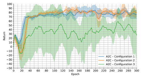
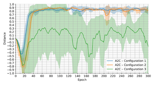
Table 1 suggests that the simplest A2C configuration has been able to achieve the most stable and thus the best average results. The fact that the variance has been a major problem for the other A2C configurations is also indicated in Figures 1 and 2, which depict the 10-epoch moving mean +/- standard deviation for the return and the distance in the evaluation episodes during training, respectively. These figures even show that the last A2C agents have been roughly the most successful for Configurations 1 and 2. On the contrary, Configuration 3 has been experiencing several performance peaks throughout the training. Lastly, all configurations have been learning fairly quickly, with very minor improvements occurring after around 60 epochs.
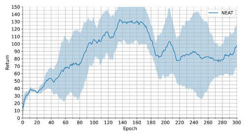
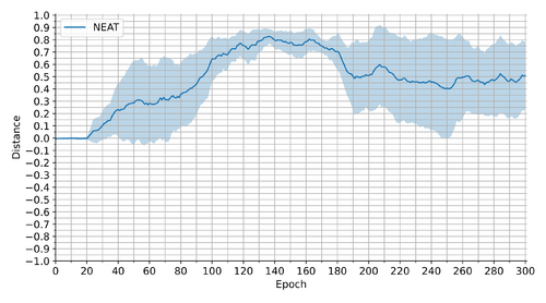
The distance information in Table 1 implies that the final NEAT agents have reached a mediocre level of proficiency compared to A2C in Configuration 1. However, they have been able to collect surprisingly more rewards through an episode, which we can see in the higher returns in Table 1. We may thus conclude that the solutions found by NEAT can avoid off-table positions better or keep the chip close to the goal for longer, but often not until the end. Unlike A2C configurations, NEAT has experienced a peak in the performance after about 140 epochs/generations, as the learning progressions in Figures 3 and 4 illustrate. This trend correlates with NEAT's qualitative regression or stagnation after that point, which we have identified by inspecting the experiment logs. Hence, we have (despite our previous intention) also tested the individuals with the best evaluation fitness among our 10-epoch checkpoints throughout the training. The results from these tests are displayed in Table 1 under the Method label "NEAT – Best". They show that the best networks found by NEAT can reach the same mean success rates as A2C in Configuration 1 in terms of the distance metric, while surpassing it in the collected return.
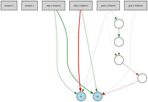
Interestingly, NEAT has managed to evolve much simpler networks, even with some input-output connections missing. Example architectures of the final agents are in Figures 5 and 6, where green and red arrows represent positive and negative weighted connections, respectively. The widths of the lines are proportional to the weight magnitudes.
Our visual assessment of the best agents' performance on the test episodes has revealed that all methods have converged to a solution where the actuator slowly pushes the chip to the goal position via circular movements, as exemplified in Animation 1. We did not expect such behaviour to be learned, instead, we thought that the actuator would push the chip directly to the goal. We hypothesize that this phenomenon may result from our friction-free, simplified simulation of chip pushing. NEAT has constructed networks with simpler approaches to the circular motion due to their lower complexity, as can be seen in Animation 2. Unfortunately, we have noticed that neither A2C nor NEAT agents can safely avoid getting off the table. More recordings from test episodes are provided in Appendix.
Conclusion
Our experiments have shown that both A2C and NEAT can be used to find neural agents that solve the considered task relatively successfully. NEAT has managed to discover simpler, but also less effective solutions than A2C. Note that we have even tried the purer NEAT algorithm without the possibility to delete connections and nodes. However, we have failed to determine the suitable values for the other hyper-parameters in that case, leading to inferior results. This experience might signal that the original NEAT would have struggled with finding a working solution.
Appendix
We provide our implementation, experimentation, and other scripts together with the logs, figures, and recordings from our experiments in the following GitHub repository: https://github.com/mousetom-sk/airob-rl-neat
References
- Sutton, R. S., & Barto, A. G. (2018). Reinforcement learning: An introduction (2nd ed.). The MIT Press.
- Eiben, A. E., & Smith, J. E. (2015). Introduction to Evolutionary Computing (2nd ed.). (Natural Computing Series). Springer.
- Stanley, K. O., & Miikkulainen, R. (2002). Evolving neural networks through augmenting topologies. Evolutionary Computing, 10(2), 99–127.
- McIntyre, A. et al. neat-python [Computer software]. https://github.com/CodeReclaimers/neat-python
